Beiträge getaggt mit Performance Tuning
Why your Parallel DML is slower than you thought
In the Data Warehouse Administration course that I delivered this week, one topic was Parallel Operations. Queries, DDL and DML can be done in parallel, but DML is special: You need to enable it for your session! This is reflected in v$session with the three columns PQ_STATUS, PDDL_STATUS and PDML_STATUS. Unlike the other two, PDML_STATUS defaults to disabled. It requires not only a parallel degree on the table respectively a parallel hint inside the statement, but additionally a command like ALTER SESSION ENABLE PARALLEL DML; Look what happens when I run an UPDATE with or without that command:
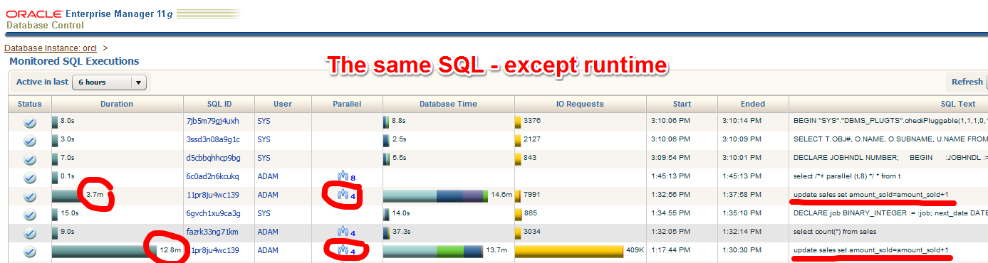 The table sales has a parallel degree of 4. The two marked statements seem to be identical – and they are. But the second has a much longer runtime. Why is that?
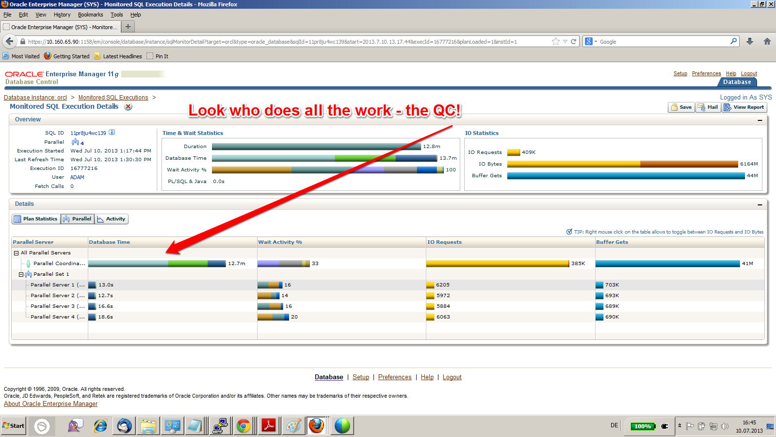 It’s because Parallel DML is disabled in that session. The fetching of the rows can be done in parallel, but the Query Coordinator (QC) needs to do the update! That is of course not efficient. The mean thing is that you see actually Parallel Processes (PXs) running and appearing in the execution plan, so this may look like it does what it is supposed to – but is does NOT. Here is how it should be, with the correct ALTER SESSION ENABLE PARALLEL DML before the update:
 The QC does only the job of coordinating the PXs here that do both, fetching and updating the rows now. Result is a way faster execution time. I’m sure you knew that already, but just in case 😉
Evidence for successful #Oracle Performance Tuning
This article shows an easy way to determine, whether your Oracle Database Performance Tuning task has been successful – or not. In the end, it boils down to „The objective for tuning an Oracle system could be stated as reducing the time that users spend in performing some action on the database, or simply reducing DB time.“ as the Online Documentation says. Best proof would be a confirmation from the end users that run time got reduced; second best is a proof of reduced DB time, which is discussed here.
A tuning task should always end with such a proof; your gut feeling or high confidence is not sufficient – or as I like to say: „Don’t believe it, test it!“ 🙂
The demo scenario: With an Oracle Enterprise Edition version 11.2.0.3, an application uses these commands to delete rows:
SQL> create table t as select * from dual where 1=2;

Table created.
SQL> begin
 for i in 1..100000 loop
 execute immediate 'delete from t where dummy='||to_char(i);
 end loop;
 end;
 /
I am pretty sure that this code is not optimal, because it uses Literals instead of Bind Variables where it is not appropriate. Before I implement an improved version of the code, I take a Baseline with Automatic Workload Repository (AWR) snapshots. On my demo system, snapshots are taken every ten minutes:
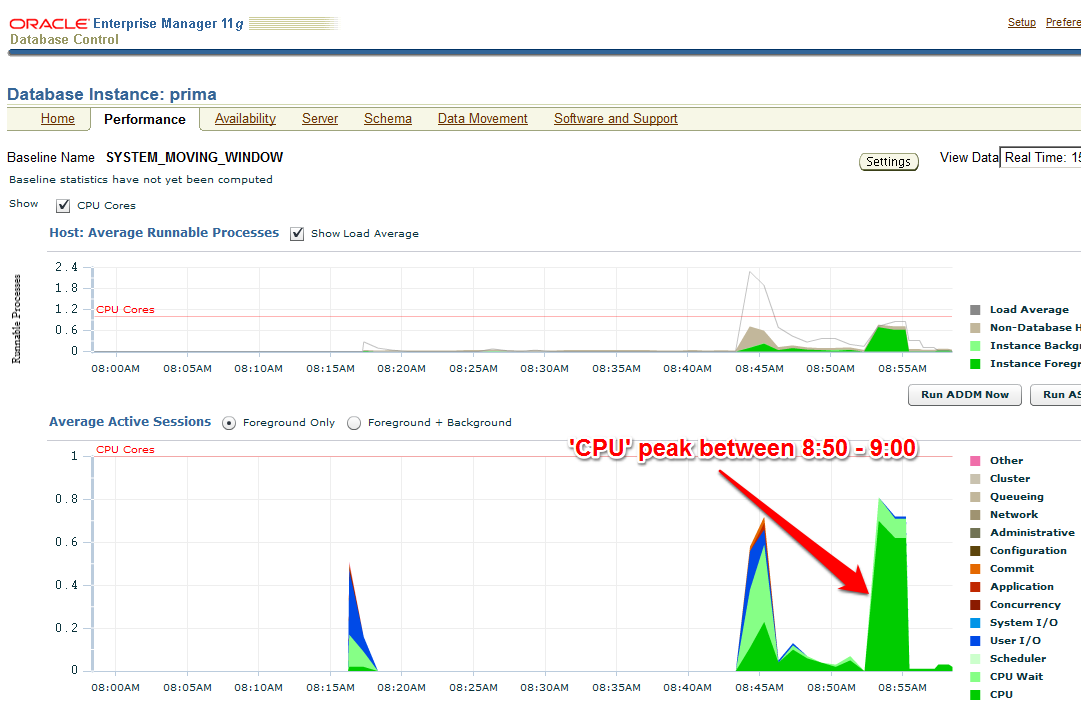
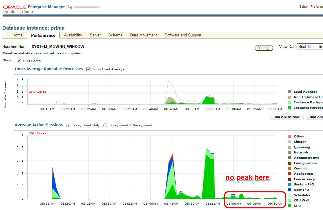
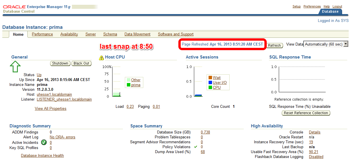 The code with Literals was just called – now about 10 minutes later on the Enterprise Manager (EM) Performance page:
 The AWR report that I take (with EM or with awrrpt.sql) as the baseline shows the following:
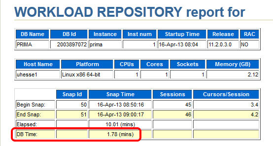 Notice especially the poor Library Cache hit ration, significant for not using Bind Variables – and the meaningless high Buffer Cache hit ration 🙂
 Starting after 9:00 am, my improved code that uses Bind Variables runs:
SQL> begin
 for i in 1..100000 loop
 delete from t where dummy=to_char(i);
 end loop;
 end;
 /
The EM Performance page show no peak during the next 10 minutes which represent my comparison period after the tuning task:
 Let’s look at the AWR report of the second snapshot range after the tuning task:
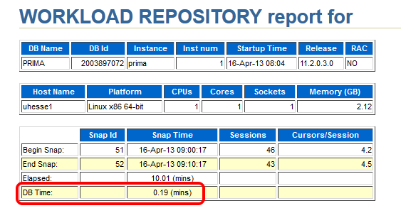 Same wall clock time, same application load, but reduced DB time – I was successful! Could stop here, but some more details:
 The important (especially for OLTP systems) Library Cache hit ratio is now very good. A very convenient way to compare the two snapshot ranges is the ‚AWR Compare Periods‘ feature in EM (or awrddrpt.sql) , which shows us instructively:
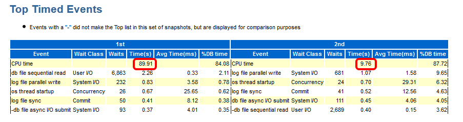
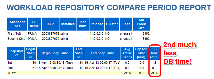 Although in both periods, CPU was the top event (also in % DB time), it took much less time in total for the 2nd period:
 The Time Model Statistics confirm a strongly reduced Parse Time for the 2nd period:
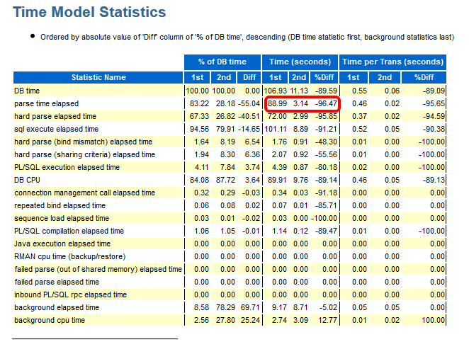 Especially, we see a striking improvement for the run time of the code with Bind Variables: From about 82 seconds down to about 3 seconds!
 This kind of proof (less DB time) can be used also in cases where the reduction of run time for a single statement is not so obvious as in my example. If 1000 users had done each 100 deletes, they would have seen not much difference in run time each – but the parse time summarizes and impacts overall performance similar as seen here. If you would like to see the three original AWR reports were I took the screen shots above from, they are here as PDFs
Conclusion: You will – and should – be able to prove the effectiveness of your Oracle Database Tuning task with a reduction of DB time from an AWR report comparison. After all, you don’t want to waste your efforts, do you? 🙂
Addendum: This posting was published in the Oracle University EMEA Newsletter May 2013
Brief Introduction into Partitioning in #Oracle
Partitioning is a great way to deal with large tables. This post will give you a quick start with examples that you can reproduce easily for yourself. Focus will be on Range-Partitioning, which is still the most popular kind.
First things first: You should only consider to implement partitioning for really large (GB range or more) objects, because it is an extra charged option and the benefits do not show significantly with small objects.
The two major reasons why you may want to use partitioning are Performance and Manageability. Let’s look at this picture:
 Above table is partitioned by the quarter. You will see that the table name and the columns are known by the application layer (INSERT and SELECT statements come from there), while the partitioned nature of the table needs to be known by the DBA only. I’m going to implement this on my demo system:
SQL> grant dba to adam identified by adam;
Grant succeeded.
SQL> connect adam/adam
 Connected.
 SQL> create table sales (id number, name varchar2(20),
 amount_sold number, shop varchar2(20), time_id date)
 partition by range (time_id)
 (
 partition q1 values less than (to_date('01.04.2012','dd.mm.yyyy')),
 partition q2 values less than (to_date('01.07.2012','dd.mm.yyyy')),
 partition q3 values less than (to_date('01.10.2012','dd.mm.yyyy')),
 partition q4 values less than (to_date('01.01.2013','dd.mm.yyyy'))
 );
Table created.
From the viewpoint of the application, this is transparent, but the value of the TIME_ID column determines into which partition the inserted rows will go. And also, if subsequent SELECT statements have the partition key in the WHERE clause, the optimizer knows which partitions need not to be scanned. This is called Partition Pruning:
 I’ll show the application perspective first:
SQL> insert into sales values ( 1, 'John Doe', 5000, 'London', date'2012-02-16' );
1 row created.
SQL> commit;
Commit complete.
SQL> select sum(amount_sold)
 from sales
 where time_id between
 date'2012-01-01' and date'2012-03-31';
SUM(AMOUNT_SOLD)
 ----------------
 5000
SQL> set lines 300
SQL> select plan_table_output from table(dbms_xplan.display_cursor);

PLAN_TABLE_OUTPUT
------------------------------------------------------------------------------------------------
SQL_ID	crtwzf8j963h7, child number 0
-------------------------------------
select sum(amount_sold) from sales where time_id between
date'2012-01-01' and date'2012-03-31'

Plan hash value: 642363238

-------------------------------------------------------------------------------------------------
| Id  | Operation		| Name	| Rows	| Bytes | Cost (%CPU)| Time	| Pstart| Pstop |
-------------------------------------------------------------------------------------------------
|   0 | SELECT STATEMENT	|	|	|	|    14 (100)|		|	|	|
|   1 |  SORT AGGREGATE 	|	|     1 |    22 |	     |		|	|	|
|   2 |   PARTITION RANGE SINGLE|	|     1 |    22 |    14   (0)| 00:00:01 |     1 |     1 |
|*  3 |    TABLE ACCESS FULL	| SALES |     1 |    22 |    14   (0)| 00:00:01 |     1 |     1 |
-------------------------------------------------------------------------------------------------

Predicate Information (identified by operation id):
---------------------------------------------------

   3 - filter(("TIME_ID">=TO_DATE(' 2012-01-01 00:00:00', 'syyyy-mm-dd hh24:mi:ss') AND
	      "TIME_ID"<=TO_DATE(' 2012-03-31 00:00:00', 'syyyy-mm-dd hh24:mi:ss')))
Notice the PSTART=1 and PSTOP=1 above, which indicates Partition Pruning. So only one quarter was scanned through, speeding up my Full Table Scan accordingly. When the table is partitioned by the day, that SELECT on a large, even filled table would run 365 times faster – which is not at all unusual, many customers have hundreds, even thousands of partitions exactly therefore.
Now to the Maintenance benefit: DBAs can now get rid of old data very fast with DROP PARTITION commands. DELETE would be an awful lot slower here – if millions of rows are deleted, that is. Or some kind of Information Life-cycle Management can be implemented like compressing old partitions. They can even be moved into other tablespaces that have their datafiles on cheaper storage:
SQL> alter table sales move partition q1 compress;
Table altered.
When you put indexes on a partitioned table, you have the choice between GLOBAL and LOCAL like on the next picture:
 The LOCAL index partitions follow the table partitions: They have the same partition key & type, get created automatically when new table partitions are added and get dropped automatically when table partitions are dropped. Beware: LOCAL indexes are usually not appropriate for OLTP access on the table, because one server process may have to scan through many index partitions then. This is the cause of most of the scary performance horror stories you may have heard about partitioning!
A GLOBAL index spans all partitions. It has a good SELECT performance usually, but is more sensitive against partition maintenance than LOCAL indexes. The GLOBAL index needs to be rebuilt more often, in other words. Let’s implement them:
SQL> create index sales_id on sales (id);
Index created.
SQL> create index sales_name on sales (name) local;
Index created.
We have Dictionary Views for everything, of course 🙂
SQL> select table_name, tablespace_name from user_tables;

TABLE_NAME		       TABLESPACE_NAME
------------------------------ ------------------------------
SALES

SQL> select table_name, partitioning_type, partition_count from user_part_tables;

TABLE_NAME		       PARTITION PARTITION_COUNT
------------------------------ --------- ---------------
SALES			       RANGE		       4

SQL> select table_name, partition_name, tablespace_name, pct_free, compression from user_tab_partitions;

TABLE_NAME		       PARTITION_NAME		      TABLESPACE_NAME		       PCT_FREE COMPRESS
------------------------------ ------------------------------ ------------------------------ ---------- --------
SALES			       Q1			      USERS				      0 ENABLED
SALES			       Q4			      USERS				     10 DISABLED
SALES			       Q3			      USERS				     10 DISABLED
SALES			       Q2			      USERS				     10 DISABLED

SQL> select index_name, tablespace_name, status from user_indexes;

INDEX_NAME		       TABLESPACE_NAME		      STATUS
------------------------------ ------------------------------ --------
SALES_ID		       USERS			      VALID
SALES_NAME						      N/A

SQL> select index_name, partitioning_type, partition_count from user_part_indexes;

INDEX_NAME		       PARTITION PARTITION_COUNT
------------------------------ --------- ---------------
SALES_NAME		       RANGE		       4

SQL> select index_name, partition_name, tablespace_name,status from user_ind_partitions;

INDEX_NAME		       PARTITION_NAME		      TABLESPACE_NAME		     STATUS
------------------------------ ------------------------------ ------------------------------ --------
SALES_NAME		       Q1			      USERS			     USABLE
SALES_NAME		       Q4			      USERS			     USABLE
SALES_NAME		       Q3			      USERS			     USABLE
SALES_NAME		       Q2			      USERS			     USABLE
This should be enough to get you started. We have much more to say about partitioning, of course: VLDB and Partitioning Guide. The pictures in this posting are from an LVC demonstration that I have done recently to convince potential customers to use this new training format, and I thought to myself: There must be something additional that I can do with this stuff 🙂
I hope you find it useful – feel free to comment, also if you’d like to share some of your experiences with partitioning that would be very much appreciated. Thank you!
Conclusion: Partitioning can be a very powerful tool in the DBA’s arsenal to transparently speed up applications and to ease maintenance. It is no silver bullet, though, so as always: Don’t believe it, test it 🙂
Related postings about Partitioning:
Partition Pruning & Interval Partitioning… shows Partitioning Pruning performance benefit with a larger table and how new range partitions are created automatically
Reducing Buffer Busy Waits with Automatic Segment Space Management & Hash Partitioning… shows why Hash Partitioning is often used for large OLTP tables to reduce contention
Partitioning a table online with DBMS_REDEFINITION… shows how to change the structure of a table while it is permanently accessed by end users
CELL_PARTITION_LARGE_EXTENTS now obsolete… shows that you get 8 MB initial extents for partitioned tables in recent versions
Partition-Pruning: Do & Don’t… shows how the SQL code determines whether Partition Pruning can be used or not
Pickleball spielen auf YouTube


