Pickleball spielen

Appliance? How #Exadata will impact your IT Organization

Veröffentlicht von Uwe Hesse in TOI am Februar 20, 2013

The impact, Exadata will have on your IT‘ s organizational structure can range from ‚None at all‘ to ‚Significantly‘. I’ll try to explain which kind of impact will likely be seen under which circumstances. The topic seems to be very important, as it is discussed often in my courses and also internally. First, it is probably useful to be clear about the often used term ‚Appliance‘ in relation to Exadata: I think that term is misleading in so far as Exadata requires ongoing Maintenance & Administration, similar to an ordinary Real Application Cluster. It is not like you deploy it once and then it takes care of itself.

Due to its nature as an Engineered System, it is partly much easier to deploy and to manage than a self-cooked solution, but there are still administrative tasks to do with Exadata, as the following picture shows:

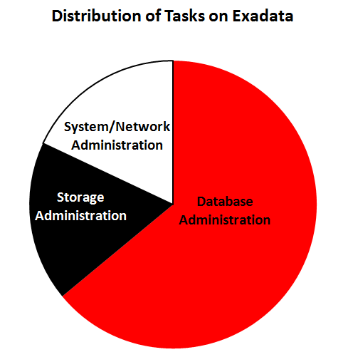Without pretending precision (therefore no percentages mentioned), you can see that the major task on Exadata is by far Database Administration, while Storage Administration and System/Network-Administration are the smaller portions. The question is now how this maintenance is done. You could of course decide to let Oracle do it partly or completely – very comfortable, but not the focus of this article. Instead, let’s assume your IT Organization is supposed to manage Exadata.

1. The siloed approach

I think it’s important to emphasize that your internal organization does not have to change because of Exadata. You can stay as you are! Many customers have dedicated and separated teams for Database Administration, Storage Administration and System/Network Administration. It is perfectly valid to decide that the different components of your Exadata are managed by those different teams as on this picture visualized:

The responsiveness and agility towards business requirements will be the same with the siloed approach as it is presently with other Oracle-related deployments at your site. There is obviously some internal overhead involved, because the different teams need to be coordinated for the Exadata maintenance tasks.

This approach is likely to be seen if Exadata is deployed more for tactical reasons (we put this one critical and customer-facing OLTP system on an Exadata eight-rack, e.g.) respectively if your internal organization is very static and difficult to change. I have seen this from time to time (SysAdmins in the course who have never seen Oracle Databases before), but I would say it is more an exception than the rule.

In short: You will get the technical benefits out of Exadata, but you will leave benefits that come from increased administrative efficiency and agility on the table.

2. The Exadata Database Administration (EDBA) Team approach

Here you give the administrative ownership of Exadata to a team, built largely or exclusively from your DBAs and give them named contacts from the other IT groups, so they can get their expertise on demand, like this picture here shows:

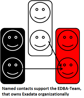Why is the DBA team supposed to own Exadata? Because as shown on Pic 1 above, they are doing the major task on Exadata anyways. And it is relatively easy to train these DBAs for Oracle Database Administration on Exadata, because they know already most of it:

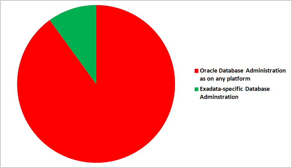I simply cannot emphasize enough how important this point is: The know-how of your Oracle DBAs remains completely valid & useful on Exadata! The often huge investment into that know-how keeps paying back! I am still surprised that the true quote ‚Exadata is still Oracle!‘ is from a competitor and not from our Marketing 🙂

For DBAs, it is similar as moving from a Single-Instance system to RAC. Some additional things to learn, like Smart Scan and Storage Indexes. Over time, the DBAs on that team may incorporate the know-how they gather at first from their named contacts of the other groups. The pragmatic EDBA approach is likely if Exadata is seen as a strategic platform, but the effort to build a DBMA team is regarded to high respectively the internal organizational structure is not flexible enough to start with the third approach. Administrative responsiveness and agility are already higher here as with the first approach, though.

3. The Database Machine Administration (DBMA) Team

Either the EDBA team evolves over time into a DBMA team or you start straight with this approach, typically by assigning some Admins from the Storage/System/Network groups to the DBMA team and let all team members cross-train in the three areas:

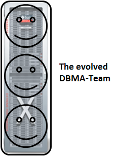This gives you the optimal administrative responsiveness and agility for your business requirements related to Exadata, which is what the majority of customers will probably want to achieve – at least in the long term. You will see this approach most likely if Exadata is supposed to be a strategic platform at your site. The good news (in my opinion) for the team members here is that they all will enlarge their mental horizon and gather new and exciting skills!

How to manage Exadata?

Regardless of your particular approach, the most important single administrative tool will be the Enterprise Manager 12C:

You can see that you can manage all Exadata components with a single, centralized tool. The picture is from our excellent Whitepaper Oracle Enterprise Manager 12c: Oracle Exadata Discovery Cookbook

Much of the above, especially the terms EDBA and DBMA can be found in our Whitepaper Operational Impact of Deploying an Oracle Engineered System (Exadata) – for some reason it is presently only available through our Oracle Partner Network. It’s kind of our official ‚party line‘ about the topic, though. I’d also like to recommend Arup Nanda’s posting Who Manages the Exadata Machine? that contains related information as well.

Finally, let me highlight the offerings of Oracle University for Exadata – you will see that there is training available for any of the three approaches 🙂

exadata

6 Kommentare

Brief Introduction into Partitioning in #Oracle

Veröffentlicht von Uwe Hesse in TOI am Januar 25, 2013

Partitioning is a great way to deal with large tables. This post will give you a quick start with examples that you can reproduce easily for yourself. Focus will be on Range-Partitioning, which is still the most popular kind.

First things first: You should only consider to implement partitioning for really large (GB range or more) objects, because it is an extra charged option and the benefits do not show significantly with small objects.

The two major reasons why you may want to use partitioning are Performance and Manageability. Let’s look at this picture:

Above table is partitioned by the quarter. You will see that the table name and the columns are known by the application layer (INSERT and SELECT statements come from there), while the partitioned nature of the table needs to be known by the DBA only. I’m going to implement this on my demo system:

SQL> grant dba to adam identified by adam;
Grant succeeded.
SQL> connect adam/adam
 Connected.
 SQL> create table sales (id number, name varchar2(20),
 amount_sold number, shop varchar2(20), time_id date)
 partition by range (time_id)
 (
 partition q1 values less than (to_date('01.04.2012','dd.mm.yyyy')),
 partition q2 values less than (to_date('01.07.2012','dd.mm.yyyy')),
 partition q3 values less than (to_date('01.10.2012','dd.mm.yyyy')),
 partition q4 values less than (to_date('01.01.2013','dd.mm.yyyy'))
 );
Table created.

From the viewpoint of the application, this is transparent, but the value of the TIME_ID column determines into which partition the inserted rows will go. And also, if subsequent SELECT statements have the partition key in the WHERE clause, the optimizer knows which partitions need not to be scanned. This is called Partition Pruning:

I’ll show the application perspective first:

 
SQL> insert into sales values ( 1, 'John Doe', 5000, 'London', date'2012-02-16' );
1 row created.
SQL> commit;
Commit complete.
SQL> select sum(amount_sold)
 from sales
 where time_id between
 date'2012-01-01' and date'2012-03-31';
SUM(AMOUNT_SOLD)
 ----------------
 5000
SQL> set lines 300
SQL> select plan_table_output from table(dbms_xplan.display_cursor);

PLAN_TABLE_OUTPUT
------------------------------------------------------------------------------------------------
SQL_ID	crtwzf8j963h7, child number 0
-------------------------------------
select sum(amount_sold) from sales where time_id between
date'2012-01-01' and date'2012-03-31'

Plan hash value: 642363238

-------------------------------------------------------------------------------------------------
| Id  | Operation		| Name	| Rows	| Bytes | Cost (%CPU)| Time	| Pstart| Pstop |
-------------------------------------------------------------------------------------------------
|   0 | SELECT STATEMENT	|	|	|	|    14 (100)|		|	|	|
|   1 |  SORT AGGREGATE 	|	|     1 |    22 |	     |		|	|	|
|   2 |   PARTITION RANGE SINGLE|	|     1 |    22 |    14   (0)| 00:00:01 |     1 |     1 |
|*  3 |    TABLE ACCESS FULL	| SALES |     1 |    22 |    14   (0)| 00:00:01 |     1 |     1 |
-------------------------------------------------------------------------------------------------

Predicate Information (identified by operation id):
---------------------------------------------------

   3 - filter(("TIME_ID">=TO_DATE(' 2012-01-01 00:00:00', 'syyyy-mm-dd hh24:mi:ss') AND
	      "TIME_ID"<=TO_DATE(' 2012-03-31 00:00:00', 'syyyy-mm-dd hh24:mi:ss')))

Notice the PSTART=1 and PSTOP=1 above, which indicates Partition Pruning. So only one quarter was scanned through, speeding up my Full Table Scan accordingly. When the table is partitioned by the day, that SELECT on a large, even filled table would run 365 times faster – which is not at all unusual, many customers have hundreds, even thousands of partitions exactly therefore.

Now to the Maintenance benefit: DBAs can now get rid of old data very fast with DROP PARTITION commands. DELETE would be an awful lot slower here – if millions of rows are deleted, that is. Or some kind of Information Life-cycle Management can be implemented like compressing old partitions. They can even be moved into other tablespaces that have their datafiles on cheaper storage:

SQL> alter table sales move partition q1 compress;
Table altered.

When you put indexes on a partitioned table, you have the choice between GLOBAL and LOCAL like on the next picture:

The LOCAL index partitions follow the table partitions: They have the same partition key & type, get created automatically when new table partitions are added and get dropped automatically when table partitions are dropped. Beware: LOCAL indexes are usually not appropriate for OLTP access on the table, because one server process may have to scan through many index partitions then. This is the cause of most of the scary performance horror stories you may have heard about partitioning!

A GLOBAL index spans all partitions. It has a good SELECT performance usually, but is more sensitive against partition maintenance than LOCAL indexes. The GLOBAL index needs to be rebuilt more often, in other words. Let’s implement them:

SQL> create index sales_id on sales (id);
Index created.
SQL> create index sales_name on sales (name) local;
Index created.

We have Dictionary Views for everything, of course 🙂

SQL> select table_name, tablespace_name from user_tables;

TABLE_NAME		       TABLESPACE_NAME
------------------------------ ------------------------------
SALES

SQL> select table_name, partitioning_type, partition_count from user_part_tables;

TABLE_NAME		       PARTITION PARTITION_COUNT
------------------------------ --------- ---------------
SALES			       RANGE		       4

SQL> select table_name, partition_name, tablespace_name, pct_free, compression from user_tab_partitions;

TABLE_NAME		       PARTITION_NAME		      TABLESPACE_NAME		       PCT_FREE COMPRESS
------------------------------ ------------------------------ ------------------------------ ---------- --------
SALES			       Q1			      USERS				      0 ENABLED
SALES			       Q4			      USERS				     10 DISABLED
SALES			       Q3			      USERS				     10 DISABLED
SALES			       Q2			      USERS				     10 DISABLED

SQL> select index_name, tablespace_name, status from user_indexes;

INDEX_NAME		       TABLESPACE_NAME		      STATUS
------------------------------ ------------------------------ --------
SALES_ID		       USERS			      VALID
SALES_NAME						      N/A

SQL> select index_name, partitioning_type, partition_count from user_part_indexes;

INDEX_NAME		       PARTITION PARTITION_COUNT
------------------------------ --------- ---------------
SALES_NAME		       RANGE		       4

SQL> select index_name, partition_name, tablespace_name,status from user_ind_partitions;

INDEX_NAME		       PARTITION_NAME		      TABLESPACE_NAME		     STATUS
------------------------------ ------------------------------ ------------------------------ --------
SALES_NAME		       Q1			      USERS			     USABLE
SALES_NAME		       Q4			      USERS			     USABLE
SALES_NAME		       Q3			      USERS			     USABLE
SALES_NAME		       Q2			      USERS			     USABLE

This should be enough to get you started. We have much more to say about partitioning, of course: VLDB and Partitioning Guide. The pictures in this posting are from an LVC demonstration that I have done recently to convince potential customers to use this new training format, and I thought to myself: There must be something additional that I can do with this stuff 🙂

I hope you find it useful – feel free to comment, also if you’d like to share some of your experiences with partitioning that would be very much appreciated. Thank you!

Conclusion: Partitioning can be a very powerful tool in the DBA’s arsenal to transparently speed up applications and to ease maintenance. It is no silver bullet, though, so as always: Don’t believe it, test it 🙂

Related postings about Partitioning:

Partition Pruning & Interval Partitioning… shows Partitioning Pruning performance benefit with a larger table and how new range partitions are created automatically
Reducing Buffer Busy Waits with Automatic Segment Space Management & Hash Partitioning… shows why Hash Partitioning is often used for large OLTP tables to reduce contention
Partitioning a table online with DBMS_REDEFINITION… shows how to change the structure of a table while it is permanently accessed by end users
CELL_PARTITION_LARGE_EXTENTS now obsolete… shows that you get 8 MB initial extents for partitioned tables in recent versions
Partition-Pruning: Do & Don’t… shows how the SQL code determines whether Partition Pruning can be used or not