Exasol introduced Partitioning in version 6.1. This feature helps to improve the performance of statements accessing large tables. As an example, let’s take these two tables:
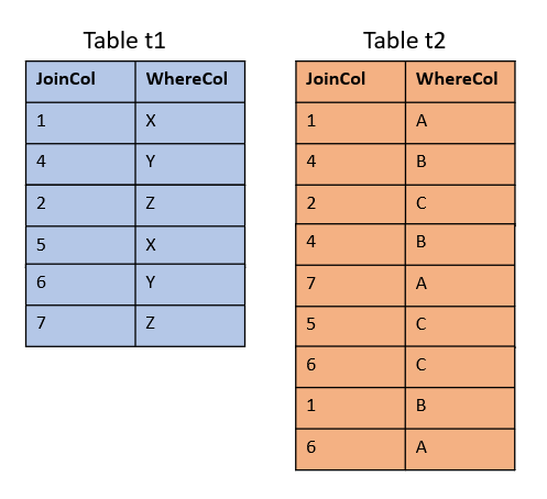
Say t2 is too large to fit in memory and may get partitioned therefore.
In contrast to distribution, partitioning should be done on columns that are used for filtering:
ALTER TABLE t2 PARTITION BY WhereCol;
Now without taking distribution into account (on a one-node cluster), the table t2 looks like this:
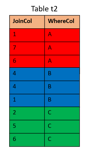
Notice that partitioning changes the way the table is physically ordered on disk.
A statement like
SELECT * FROM t2 WHERE WhereCol=’A’;
would have to load only the red part of the table into memory. This may show benefits on a one-node cluster as well as on multi-node clusters. On a multi-node cluster, a large table like t2 is distributed across the active nodes. It can additionally be partitioned also. Should the two tables reside on a three-node cluster with distribution on the JoinCol columns and the table t2 partitioned on the WhereCol column, they look like this:
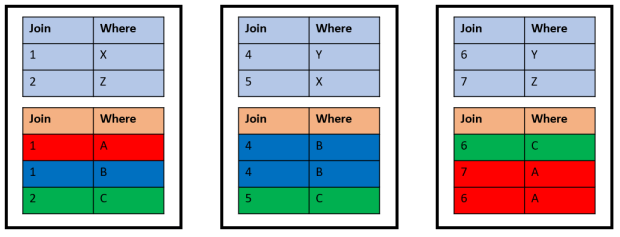
That way, each node has to load a smaller portion of the table into memory if statements are executed that filter on the WhereCol column while joins on the JoinCol column are still local joins.
EXA_(USER|ALL|DBA)_TABLES shows both the distribution key and the partition key if any.
Notice that Exasol will automatically create an appropriate number of partitions – you don’t have to specify that.

